Geosonnet 65

Speed dating is a scattershot affair
Which blasts the hearts of river zircon grains
No magic mirror can discern the fair
And youngest zircon sediment contains.
If dating based on chemistry is used
The youngest grain is easier to find.
But chemistry is tedious! Abused
Statistics can be questioned and refined.
The youngest kernel density’s a crone
The youngest single grain is way too young,
Statistical young grouping’s in the zone
Though less exacting than the dates Tims’s brung
So settle down, this zircon dating’s docile
Until you try to match it with a fossil.

Geology 47 1044

Other geosonnets: 1 2 3 4 5 6 7 8 9 10 11 12 13 14 15 16 17 18 19 20 21 22 23 24 25 26 27 28 29 30 31 32 33 34 35 36 37 38 39 40 41 42 43 44 45 46 47 48 49 50 51 52 53 54 55 56 57 58 59 60 61 62 63 64  65 66  67 68 69

Geosonnet 55

A plotter’s pause to synchronize his watch

Is often preparation for a heist:

A bank vault? Tardy mail train full of scotch?

A drug syndicate’s freighter full of ice?

Geologists scheme on a grander scale

Where ice envelops Earth, a mile thick.

Should cryospheric pilfering prevail

The melting must be synchronous, and quick.

Boron reveals (in sonnet twenty five)

Cap carbonates have one last common flaw

A rapid deposition crooks derive

A catastrophic warming's last hurrah

   The zircons say less than a million years.

   CO₂ melts the ice, then disappears.

Geology 47 251

Other geosonnets: 1 2 3 4 5 6 7 8 9 10 11 12 13 14 15 16 17 18 19 20 21 22 23 24 25 26 27 28 29 30 31 32 33 34 35 36 37 38 39 40 41 42 43 44 45 46 47 48 49 50 51 52 53 54 55

Routine science turns clever- laser ICP vs SHRIMP analysis of Archean detrital zircons

So, last year I published a Geology paper. It is summarized in Geosonnet 42; see link therein to the paper itself. As it turns out, the paper deals with Archean uranium mobilization and the sedimentary history of carbonado diamond. But what the paper doesn’t say is that I wasn’t actually trying to do that. More professional researchers than I might know how state in their articles that it was all just a lucky coincidence, but I don’t know how to squeeze that into a short format journal.

What actually happened is that the second author and I realized that we had different pieces of the puzzle which, with the help of some old Japanese data, could be pieced together for a coherent story. So hey, "write it up."  Most of my part of the puzzle was unpublished bits and pieces from my PhD and post doc 15+ years ago, but the SHRIMP data was actually less than a year old, as I had collected it for an entirely different reason.

Back when I was working at ASI, which had just bought the Resolution laser ablation line from Resonetics, a few of us started looking at how the SHRIMP and laser products could best compliment each other. One of the things we experimented with was controlling the SHRIMP with a version of the laser control software. Another thing we wanted to know was whether there was any advantage to using the SHRIMP for detrital zircon provenance studies, so I pulled out my old PhD zircons, remounted them with modern standards, and we programmed a customized version of GEOSTAR to automatically rerun the same zircons (if they hadn’t been blown up) to compare the results. Of course, the laser data was old, and the SHRIMP was trying to make analyses next to laser holes (which distort the extraction field, due to the unfortunate tendency of holes not to be flat), but it generally worked, and the data is tucked away deep in the supplementary section of the paper.

Since there are analytical geochemists who occasionally read this blog, but might not think to look for microbeam comparisons in the appendix of a diamond radiation defect luminescence paper, I thought I’d mention it, and put up some plots that got culled due to space requirements.

The short answer is that fully metamict zircons (like half of the Tombador grains) are open system with either technique, but for zircons that are only a little bit metamict (most of the Jacobina zircons), the smaller ion probe spot and better ²⁰⁴Pb backgrounds improve data quality. Anyone who is interested is welcome to download the Data Repository data (it’s all there) and ask.

Figure 1 (See data repository for full version): Tombador zircon analyses with SHRIMP (red) and laser ICPMS (yellow). The SHRIMP data are, in general, a little more concordant, but there isn’t much in it.

Figure 2 (See data repository for full version): Jacobina zircon analyses with SHRIMP (red) and laser ICPMS (yellow). For this sample, the SHRIMP data are substantially more concordant.

Figure 3:  Probability distribution curves for Tombador zircons analysed by SHRIMP (purple) and laser (Red).

Figure 4:  Probability distribution curves for Jacobina zircons analysed by SHRIMP (tan) and laser (Red). Note that laser peaks are generally broader and offset to younger ages due to Phanerozoic Pb loss.

Effect of impact energy on SIMS U–Pb zircon geochronology

I have a paper out in pre-publication online availability. The basic gist of it is that we are investigating exactly why SHRIMP is so good at geochronology.  It is a short format conference proceedings paper, so there isn't that much to it.  Basically, we investigated the oxide formation used to calibrate relative U/Pb ionization yields by bombarding natural zircon with a primary ion beam made of ¹⁸O₂^- ions.  This way, all the molecular oxide ions were isotopically labeled- ¹⁶O if the oxygen originated in the sample, ¹⁸O if it was from the primary beam.  We then varied the ion impact energy to see what effect this had on the overall collection efficiency.

One of the other different things about this paper is that I co-wrote it with my dad.  He doesn't know any geology, but since I was about five he has been using SIMS (not SHRIMP, other brands) analysing semiconductors.  He still lives in America, so I don't get to see him much any more, and he's not getting any younger.  So it was nice to have a structured activity to work on together.  The middle author, Jim Ferris, did the atomic force microscopy. Unfortunately due to the short format, we didn't have space for any of his pictures, but he measured the sputter crater volumes, which we needed to calculated useful yields.



Magee C. Jr., Ferris J. and Magee C. Sr. (2014), Effect of impact energy on SIMS U–Pb zircon geochronology, Surface and Interface Analysis, DOI: 10.1002/sia.5629

Bayesian Geochronology

 Bayesian statistics is a growing field of exploring data-rich, complicated, explanation-poor phenomena. In a nutshell, you start out with an initial assumption, called a “prior” and then modify it with new sets of independent data. The Bayesian approach is one of the hot new techniques to come into Earth Science in the past decade, as it allows us to sensibly integrate disparate sets of data about the same physical process derived from different proxies or fields. Long time geobloggers will know that James is an expert in applying this technique to climate; see his blog and papers for more information.  However, despite the decade-long use in climate science, Bayesian statistics have not often been applied to more interesting areas of geoscience.  E.g. Geochronology.  Until now.

In Geology, Vleeschouwer & Parnell present a new Bayesian method of constructing the geologic timescale.  They point out that the previous timescale, which were just spline fits between selected stratigraphic/geochronological time points, had the perverse effect of yielding smaller error bars in the gaps between data points than near to where there are data. So they try a Bayesian approach instead.

For their Prior, they start off with the rule of superposition- which states that lower stratigraphy is older than higher stratigraphy.  They then apply all the high precision geochronology dates (high-precision CA-TIMS U-Pb in this case), and generate a probability density function for stratigraphy vs time. Their resulting chronology is, sensibly, more erroneous in areas where there is no data, compared to those where data does exist.  But in addition to being more sensible, this approach is far more useful.

Firstly, from the modeled uncertainties in the interpolated regions, one can guestimate the precision (both geochronological and stratigraphic) that is necessary to help constrain the timescale.  So, for example, in some of the more data-poor regions, one can probably usefully constrain the timescale using a less precise microanalytical method such as SHRIMP, if the only available zircons are not suitable for CA-TIMS.  On the other hand, as you approach a high precision date, lower precision techniques become less useful.

In fact, you can tell whether or not a particular age is useful for the timescale simply by looking at how the inclusion of that date alters the PDF.  Previously, the inclusion or rejection of particular ages has been a non-transparent potentially politicized process.  The use of this model allows us to replace the argumentative old men with statistics.

Of course, one needs to be careful in adding data.  A potential flaw would be adding lots of data with a systematic error (for example, of there are still lingering systematic issues with U-Pb vs Ar-Ar dating, or the offsets in some zircon ages dated using laserICP by Gehrels et al. 2008). But one thing this method does allow is the addition of different types of data.

Vleeschouwer and Parnell (2014) demonstrate this in the second half of their paper, using astrochronology.  This is the appearance in the sedimentary record of depositional changes that are related to Milankovic cycles- the changes in the Earth’s orbit that govern, for example, the extent of ice sheets in the modern Earth.  Astrochronology cycles do not add additional tie points to the geochron/stratigraphy tie curve, as they are relative dates with no fixed reference.  However, what they can do is constrain the slope of the line.  So changes in stratigraphic distance between periodic eccentricity cycles tells us how the stratigraphic progression changes with time, often on a much shorter timescale than what we can access using traditional U-Pb geochronology.  The Bayesian approach allows us to integrate the strengths of both methods, giving a more accurate and reliable timescale.  

Argon-Argon Dating: The Simple Version

  Sciency Thoughts has a post up on recent high-precision ³⁹Ar/⁴⁰Ar dating of the Toba supervolcano in Indonesia.  Unfortunately he seems a bit confused about the technique.

Argon has three naturally occurring isotopes: ³⁶Ar, ³⁸Ar, and ⁴⁰Ar. Potassium also has three isotopes, ³⁹K, ⁴⁰K, and ⁴¹K.  One of these isotopes, ⁴⁰K, is radioactive, with a half life of about 1248 million years, and one of its stable decay products is ⁴⁰Ar.

 In the universe, and in Jupiter and the Sun locally, ³⁶Ar is the most abundant argon isotope, followed by ³⁸Ar.  In the cosmic scheme of things, ⁴⁰Ar is so rare that we don’t even know what its overall abundance is.

However, Earth is a rocky planet.  It was not able to hold onto much gas during its formation, so there is very little ³⁶Ar and ³⁸Ar here.  Earth has lots of potassium though, so almost all the Ar in the atmosphere is ⁴⁰Ar, which is the decay product of ⁴⁰K.

In a potassium-bearing mineral, the ⁴⁰K decays into ⁴⁰Ar, so you can measure the ratio of these two isotopes to figure out how old the mineral is.

The problem is that it is technically very difficult to measure a potassium argon ration accurately, because one is a reactive solid, and the other is an inert gas.  They require different sorts of ion sources, different mass spectrometers, and there are all sorts of chemical effects that complicate the measurement.

If you want an accurate ratio, it is much easier to measure isotopes of the same element.

So for ³⁹Ar-⁴⁰Ar dating, what happens is that the mineral of interest is put into a nuclear reactor and bombarded by neutrons.  Some of the ³⁹K (the most abundant stable potassium isotope) absorbs a neutron, ejects a proton, and transmutes into radioactive ³⁹Ar.  ³⁹Ar has a half-life of a few hundred years, and is virtually non-existent in nature.   So as long as you know your nuclear ³⁹K to ³⁹Ar conversion ration well, this method allows you to use the ³⁹Ar as a proxy for ³⁹K.  The handy thing is that because it is argon, not potassium, it behaves chemically just like the other naturally occurring argon isotopes, so you can measure it in a gas source mass spectrometer much more accurately than you can measure the chemically different ³⁹K and ⁴⁰Ar.

The initial ³⁹K-⁴⁰K ratio doesn’t very much in nature, and is taken as constant (I think- I’ve never actually done Ar-Ar). But the take-home point is that ³⁹Ar-⁴⁰Ar dating is not its own decay system.  It is the ⁴⁰K-⁴⁰Ar decay system, but using a nuclear reactor to change some of the potassium into an unstable argon isotope to make the nuts and bolts of measuring it easier. 

Jailbait zircons

As the company SHRIMP driver, I do a fair bit of demonstration analyses for potential customers.  One thing that has become increasingly common over the past two years is demonstration of the ability to successfully date jailbait zircons.  For those of you unfamiliar with the term, a jailbait zircon is a zircon so young that dating it while making all the usual assumptions will get you into all sorts of trouble. 

The chief problem is that for deep geologic time, we assume that the ²³⁸U to ²⁰⁶Pb decay is a simple process. In actuality, there are eight alpha decays and more beta decays than I can remember in this process, but most of the intermediate daughter products are short-lived relative to the age of the analyst, much less the Earth.

However, if you are dating a phase that is much, much younger than the Earth, then these intermediate decay products can become important.  Corrections need to be made relating to whether or not now-extinct intermediate species were incorporated into the target mineral more or less efficiently than uranium. 

For minerals which are a few hundred thousand years old, or younger, you can abandon the uranium-lead system entirely, and use uranium-thorium dating instead.  This simply looks at how close to secular equilibrium ²³⁰Th and ²³⁴U have grown after their initial incorporation into the target mineral in a unequilibrated ratio.  The linked wikipedia explanation is good (at least qualitatively).  Check it out.

Of course, even for targets old enough for uranium-lead dating, in addition to the theoretical problems above, there is the practical problem of measuring a statistically significant amount of very low levels of radiogenic lead, while somehow keeping common Pb contamination to an absurdly low level.  Because one of the nasty things about the disequilibrium species is that they disrupt many of the assumptions that are needed to accurately and precisely correct for common lead.  Which means that if you can’t keep the blank down, you’re screwed. 

Pre-Proterozoic Political Proletariat

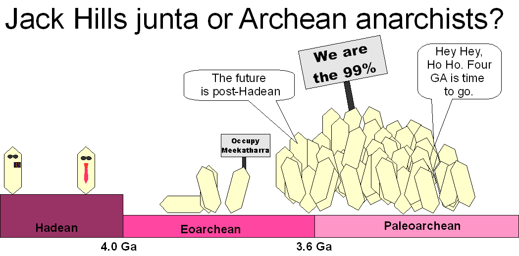
For those not familiar with old Earth geology, the conglomerates of the Jack Hills contain detrital zircons, and the 1% of those zircons which are older than 4 billion years consume 95% of the resources used to study these mineral grains. Clearly, this is the longest-running example of economic inequality on this planet.

Isaac Asimov describes uranium-lead geochronology

Cleaning out some old filing cabinets here at work, I found some old newspaper clippings of a science article by Science Fiction and popular science writer Isaac Asimov, describing uranium-lead geochronology of zircon.

As it turns out, the article still exists in the on-line archive of the LA times.  It can be found here.  Although the article is 22 years old, neither the fundamental physics, nor the billion-year-old rocks, have changed much during that time.  So it is still a useful reference for anyone wanting to know the basics of uranium-lead geochronology, and early earth history.

Early Earth awesomeness and middle Earth magic

One of the problems with making illustrated linear geologic timescales is that the middle 80% of the timescale generally looks fairly boring. Of course, all sorts of things were happening in the Archean and Proterozoic, but they ren't always as easy to sketch cartoons of as a trilobite. I'm currently doodling a cartoon illustrated timescale, and I was wondering. do any of you have any favorite Precambrian events that can take up the timeline space that would otherwise be white? If so, and you don't mind me stealing your favorites, please share.

How long as the Atacama been dry?

“I am flying home from Europe in late August with nothing but a notebook and the 2011 Goldschmidt conference Geology giveaway issue to keep me occupied. Using the old-fashioned method of reading and writing on paper, I will blog my way through the compilation of highlighted geochemistry papers as time allows. These will then be posted via time delay to keep the blog moving while preventing paper burnout.”

The Atacama desert, on the west coast of South America, is the driest desert on Earth. The high Andes mountains block moisture transport from the Amazon basin, and the cold Humboldt current offshorehttp://www.blogger.com/img/blank.gif provides little evaporative moisture.

Dunai et al. (2005) attempt to determine whether the hyperarid conditions are ancient (early Miocene) or more recent (late Miocene) by looking at the cosmic ray exposure ages of easily eroded sediment.

Cosmic rays are extremely high energy protons which are generated beyond our solar system (ask an Astronomer for details). The are energetic enough to penetrate the atmosphere and the first few meters of rock when they strike the Earth. When they do hit rock, they can create nuclear reactions between the atoms in the rock. One of the products of these reactions, ²¹Ne, can be measured using noble gas mass spectrometry. So the amount of excess ²¹Ne a rock has is proportional to how long it has been close to the earth’s surface, and the cosmic ray flux.

Dunai et al. (2005)’s sample sites were specifically chosen to exclude areas where the outwash from the high Andes east of the desert would erode or cover the local rocks. Only local rainfall could erode the selected areas, so only local, medium elevation, near-shore precipitation (or lack thereof) was relevant to the erosion rates.

Their results show that most of the rocks they sampled have been at or near the surface for 20-30 million years. These are among the oldest exposure ages in terrestrial rocks. The implication is that there has been negligible erosion since that time.

On the other hand, I wish the paper made more of an effort to explain why the results given were not within error of each other. Call me old fashioned, but a data table would be nice as well.

The other question that they ask is which came first, the aridity or the uplift? It is easy to see how uplift causes aridity- the rain shadow gets stronger. How aridity causes uplift is less obvious, and the reference given is not available on this aircraft. But the general idea (based on context) seems to be that with no fluvial input to the subduction trench, it accumulates very little sediment. Without sediment, the rocks are stronger, and can withstand more stress, pushing the mountains higher.

The problem with this conclusion is that it requires knowing the sediment flux from the entire drainage area. Presumably the sediment transport would be controlled mainly by erosion of the high (and higher precipitation) Andes.

Dunai et al. (2005) specifically chose a site that did not record the sediment flux from the eastern, mountainous part of the drainage basin. Instead they chose to focus on local conditions. By excluding the most important potential sediment source, they put themselves in the worst possible position to answer questions about sediment transfer in the rest of the Atacama desert, including total transport to the trench.

Dunai, T., González López, G., & Juez-Larré, J. (2005). Oligocene–Miocene age of aridity in the Atacama Desert revealed by exposure dating of erosion-sensitive landforms Geology, 33 (4) DOI: 10.1130/G21184.1

Wasting time on the internet?

Looking for something to read? Sorry, I'm running a mass to field calibration so that my isotopes appear at the correct apparent mass for tomorrow's visitor. I can't entertain you this evening. But if you're thinking you might want to do something vaguely useful to society, and you know something about geology (and I know a lot of y'all do), head over to Wikipedia's WikiProject Geology and see if you can apply your expertise to educating the world. It will be far more interesting than determining that mass 238.051 amu is centered in the detector when the magnet has a field value of 2219.269 gauss. Trust me. I'm thrilled because I'm starting at the top of the table and working down.

Sphene

Is my favorite geological word. Or rather, my favorite formerly geologic word. From a lawyeristic point of view, it hasn’t been a geologic word since 1982, despite having been the preferred name for Ca TiSiO₅ for the 4,566,999,971 years prior to that date. These days, you don’t sphene spoken of much, as most of us who mutter it are busy yelling at the young whippersnappers to get off our psilophytopsid lawns. However, it has not totally disappeared from the scientific literature, despite the best efforts of the IMA to discredit it. And the materials scientists might actually still prefer sphene (God belss them).

Of course, most mineralogists these days dutifully go along with the official name (the “T-word”, since despite my use of cunt, nigger, and fuck in this blog, I do draw a line at really offensive words, like t*&#%ite). And why shouldn't they use the official name? They are just following orders. But there are still a few cowboy rock smashers around who got into this field because we were never particularly good at following the rules. And while I am not so old-fashioned as to refer to element 41 as columbium, I do prefer sphene.

The T-word is a stupid name. The mineral was known (and called sphene) long before the element titanium was discovered. The name is derived from the greek word for wedge, whoich describes the shape perfectly. In contrast, commercial titanium is mined from ilemite or rutile, not sphene. And the element was originally discovered (independently) by processing ilmenite (in the UK) and rutile (in Germany) in the 1790’s.

Sphene has a domain name.
The t-word does not.
Sphene is pretty.

Finally, any sphene used in geochronology was almost certainly sphene when it crystallized, and only morphed into the T-word at a very late stage in its evolution. Fortunately, the sphene/T-word transformation does not upset the U-Pb isotopic system, so that dating of sphene is still possible today.

Born again zircons

Last summer, I spent a bit of time back at Geoscience Australia as a geochronologist for hire, helping out with some of their state and territory geochronology programs. The report from the study I SHRIMPed zircons for is now out, thanks to the awesomeness of the first author, Dr. Nat Koscitin.

In theory, zircons are forever. The oldest known Earth materials are zircons, and there are countless* papers describing how they accumulate overgrowths through numerous heating and melting events.

So I was intrigues when I saw the following embayments on one of the samples. It is obvious that the zircon structure has been altered somehow. Prior to analysis, I assumed that it would be metamict- zircon where the accumulated radiation damage has destroyed the mineral structure.

Embayed zircons (c) Geoscience Australia

Usually, metamictization allows the radiogenic lead to escape, leading to geologically meaningless uranium-lead ratios. So I was surprised when these inliers gave a beautiful age that was 25 million years (plus or minus five) younger than the igneous crystallization age.

Igneous ages (red) are distinctly older than embayment ages (blue), which are surprisingly (to me) tightly clustered (c) Geoscience Australia.

The inliers have very low, “metamorphic type” Th/U ratios, suggesting that the zircon was drastically recrystallized, if not completely destroyed and regrown. These zircons weren’t forever; they had their insides dissolved and reprecipitated when they were 25 million years old. I had a brief look through the literature, but didn’t find anything that looked particularly similar. So I flicked the interpretation back to the petrologists and/or fieldies in the text. They didn’t come to the rescue- at least not yet.

If anyone knows how these things form, what they mean, and where I can read about previous descriptions, I’d appreciate it. I hear that the Curtin University gang has seen something similar, but I don’t have a particular reference. Any tips out there?


* Well, hundreds at least

What does TEMORA stand for?

Ion probe (or SIMS) geochronology has no shortage of acronyms. SHRIMP is the most obvious one, and that in turn has spawned a number of associated abbreviations, such as PRAWN, ZOC, and the various standards (QGNG, FC1, SL13 BR266, etc.). In SHRIMP (and other SIMS- CAMECA stands for something in French) analysis, standards are used because the ionization efficiency of both Pb and U is variable, so you need something with a known Pb/U ratio to correct for these effects. One of the current popular standards is called TEMORA.

So I shouldn’t have been surprised when an American visitor to the RSES at the ANU asked me what TEMORA stood for. I wish I had a snappy answer. Perhaps he was expecting something like

Thermally Equilibrated Magnetite-Orthoclase Rhyolitic Assemblage*

Or

Time Evidently Made One Resplendent Anchorpoint

Or

The Excellent Mother Of Radiogenic Architypes

Because the boring truth is that it doesn’t stand for anything. Temora is the name of a town in Western NSW. The standard comes from a specific outcrop of the Middledale gabbroic diorite, and the particular outcrop from which this zircon was extracted happens to be on the road to Temora. Like most sources of zircon standards, this is an evolved mantle melt.

Crustal rocks are generally not chosen for zircon standards, as the zircons in crustally derived igneous rocks have a greater chance of being inherited from the source rock. This would make them older than the igneous zircons, giving your ‘standard’ two populations with different ages. This particular gabbroic norite from the fields near Temora was found to be fairly well behaved, isotopically speaking, so it has been widely used as a U/Pb, Hf isotope, and oxygen isotopic standard.

As for the town of Temora, it is a small country town in winter wheat and sheep country. It’s main claim to fame is the aviation museum, which keeps a number of vintage aircraft in flying condition and occasionally puts on shows.

The Temora zircon was called TEMORA 1 in the paper that originally described it. I have no idea why it was capitalized in this way. But it’s not an acronym. Perhaps the author just needed to yell to be heard from that far out in the bush.

* This would be wrong: It’s a gabbroic diorite.

Young rocks

Evy, the skepchick who is now geoblogging at georneys, recently expressed surprise at a paper which labeled rocks with an nine digit age as young. I see nothing wrong with this, however. Depending on how you define 'beginning', the Earth is between 4567 and 4460 million years old. using 4500 as a convenient round number, we can then take half that as a midpoint, and place the old rock / young rock divide at 2250 MA. Alternatively, we could lash out and use 1.5 billion year divisions to call rocks old (> 3.0 Ga), middle-aged (between 3 and 1.5) and young < 1.5 billion.

In Gondwanaland, the 1.2-1.0 Ma Grenville orogeny is much less prevalent than it is in laurentian rocks. It shows up here and there, but is not a major event. The middle proterozoic was in fact fairly quiet in Gondwana, with the Neoproterozoic-to-Cambrian Pan-African / Brasiliano / Ross orogens being the defining tectonic events that assembled the various pieces of Gondwanaland into the supercontinent that we all know and love. So for those of us interested in the pre-assumblage history of Gondwana, it makes perfect sense to describe anything after the midproterozoic as young. I even did so in my thesis, in this sketchmap of the geology of the Brazilian state of Bahia:

Detrital minerals done right

This afternoon, I got to go listen to a talk by Andy Morton. As anyone who hangs around the geochronology scene for any length of time knows, detrital provenance studies are done often, with a wide variety of quality and rigour. The basic idea is that you can learn about the source region of a sand by looking at the individual grains. How much you learn, and what sort of study is most informative, is something that isn’t always clear, as this is a field of study where the wheel is reinvented often and badly. The basic idea is so simple that people don’t often spend oodles of library time looking at how the field has evolved over the decades. So it was really cool to listen to the guy who has been at the forefront of doing detrital studies well for the last 30 years.
Like much great science, the talk was deceptively simple. He started out explaining the various sedimentary processes that give rise to sample bias, specifically diagenesis, transport, and weathering. He then went through the heavy mineral ratios, and the chemistry of each one- what the garnet chemistry tells you, what the tourmaline chemistry means, etc., through the entire mineral suite. Only after that did he get into geochronology. And each piece of the puzzle fell together- the tourmalines identified the granite types, the rutiles identified the high grade metamorphic conditions, the garnets identified the medium grade metapelites and deep crustal rocks, the zircons gave the ages. Occasionally spinels would make mafic igneous cameos. As it came together, the picture of the source would suddenly congeal- Of course that combination of X metamorphism and Y plutonism at time Z was from source region W- once all the pieces are assembled, it’s perfectly clear.
And once the provenance is determined, the alteration overprint on the source assemblage in various sands of similar derivation can be used to determine burial temperature, source weathering, flood plain behavior, and a host of other paleoprocesses that most detrital mineral amateurs don’t even begin to consider. It was awesome.

Geochronology of the Cryogenian glaciations

A few weeks back Chris posted a lovely writeup of his work on the Oman cryogenian diamictites, and the snowball earth hypothesis. A recent paper on some Chinese diamictite ages has a nice summary of the chronology of this time period, so I thought I would throw it up here.

First, a short introduction. Between about 750 and 580 million years ago, a number of glacial sediments appear in the sedimentary record. Some of these appear to have been deposited fairly close to what was the equator at the time, and it was hypothesized that this may have been evidence for the planet having completely frozen over- a scenario known as the “Snowball Earth”. Subsequent stratigraphy identified three or four potential episodes of worldwide glaciation.

One of the ways of testing this theory is to see if all of the glacial strata assigned to a particular episode were actually deposited at the same time. Because there were no widespread diagnostic fossils this early in Earth’s history, biostratigraphy is not an option. One method used is to look at isotopic excursion in the sediments, on the assumption that they reflect a global signal, and not a local phenomenon. Another approach is to use radiometric dating to constrain the ages.

The problem with a radiometric approach is that there are relatively few sedimentary minerals that can be dated directly. So one generally looks for volcanic ash beds, crosscutting dykes, or other igneous rocks with an unambiguous relationship to the sediment in question. If these exist, then you can bracket the sediment in question with older-than / younger-than relationships.

There are several methods used to determine radiometric ages of neoproterozoic rocks. The most widespread is SHRIMP U/Pb geochronology. This method directly analyses the mineral zircon from igneous rocks of interest. Its advantage is that it is an in-situ method that only analyses a small portion of the grain, so it can be used on a wide variety of zircon crystals. The disadvantage is that achieving accuracy of better than 1% is difficult.

Another increasingly common method is CA-TIMS. In this method, zircon minerals are leached to remove damaged parts of the crystal, thin dissolved in acid and run on a traditional thermal ionization mass spectrometer. The advantage of this method is that it is much more accurate. The disadvantage is that it requires higher-quality zircons; inclusions and multiple growth episodes are more problematic.

A new method starting to be used is black shale Rhenium-Osmium dating, which directly dates the sedimentation of disseminated molybdenite in anoxic shales. This method should have similar accuracy to SHRIMP, but it is new enough that there could be unforeseen issues with its widespread application.

Neoproterozoic rocks have generally been metamorphosed since deposition, so K/Ar dating is usually not applicable.

In this paper, Xu et al. determine the age of three ash layers within a diamictite sequence using SHRIMP U-Pb geochronology. They then compare their results to those taken from allegedly correlated units from around the world, and those comparison charts (their figure 4) are shown below.

The following figures are laid out sideways, with older to the right. The lines represent the uncertainty in the measurement; the yellow arrow represents the relative age of the dated rock to the glacial event: younger, older, or synchronous.


As can be seen from the Gaskiers results, literature values do not contradict the existence of a short-lived, synchronous glaciation in the 580-590 Ma range. This study does not further refine this constraint, but the measurement is consistent with Xu et al’s uppermost unit being a Gaskiers correlate.

The Elatina/ Nantuo event is more commonly referred to as the Marinoan glaciation. However, the Marinoan rocks, in South Australia, have very poor age constrains, while the Nantuo is very well constrained.

So when testing for synchronicity, the Nantuo is a more sensible reference (in fact, it may be the golden spike). Once again, the Xu data does not shed much light on this event, but previous data does not contradict a single event in the 643-635 age range.

Finally, we get to the Sturtian. As is shown in this figure, ages for the glacial rocks below the Marinoan glaciation are all over the place.


Xu’s data is no exception; His data indicate a prolonged period of glaciation that precedes most Sturtian-aged rocks from other locales. As an examination of previous Sturtian work shows, a single world-wide Sturtian event is only allowed under the following conditions:
1. It is very long- with a minimum length of 40 million years.
2. It gradually thaws, with some areas deglaciating and precipitating carbonate caps tens of millions of years before other areas.

An open-access copy of the full paper can be found here.
XU, B., XIAO, S., ZOU, H., CHEN, Y., LI, Z., SONG, B., LIU, D., ZHOU, C., & YUAN, X. (2009). SHRIMP zircon U–Pb age constraints on Neoproterozoic Quruqtagh diamictites in NW China Precambrian Research, 168 (3-4), 247-258 DOI: 10.1016/j.precamres.2008.10.008

GSA meeting presentations

One of the reasons I have not been blogging much recently is that I have been spending too much time on the internet for work. Much of that involved collating research done using our instruments that is being presented at the conference. So for anyone interested in applications of zircon geochronology to geologic problems, I have a list.
And, yes. The time scale is correct to within a pixel, and uses the international standard colors. It is the ICS timescale, though, not the GSA one.

Naughty Geology

A few months back, I blogged about the client with a spam filter so tight that it embargoed emails about single young zircon dating. After conferring with said clients, it turns out that they’ve had other issues as well. In its animatronic zeal to rid the internet of pornography, this filter also blocks image files that it suspects are explicit. What sort of images? Well, anything containing a lot of pink, as it turns out. So, rose quartz, rhodocrosite, Mg-rich garnets, and other titillating mineral images have been known to disappear into the computer program’s private locker. Luckily they ship geologic maps as GIS files instead of images, or I’m sure they’d be targeted as well.

This got me thinking. How common are explicit geologic formations? You’d think that will all the zillions of folded, rounded, curved, or protruding structures on this planet, at least a few would be shaped like something that would constrict the coronary arteries of a shrill old censor. So, this is my challenge to the blogosphere: Find juiciest, most risqué geologic image that you feel comfortable posting, and put it out on the internet. Your traffic in tragically maladjusted lapidarians will expand tremendously, I guarantee.

Sadly, all I can offer in this department is this backscattered electron image of a rutile. To most people, it is simple igneous compositional zoning of Nb, Sn and W, which reflect electrons more efficiently than titanium and therefore appear bright. But to the dirty regolithic mind, this only needs legs, arms, and a head to become a swimsuit model. And no, I don’t need to leave the lab more often.


Figure 1. Detrital Phanerozoic rutile believed to be of pegmatitic origin See Birch et al. 2007 for geochronology and trace element characteristics.